How to Build Simple Image Classifier (torch, torchvision, CIFAR)
Image Classifier with CIFAR-10

An image classifier is a machine learning tool that can identify different items in pictures. To create one, we need to give a neural network lots of images that have labels. PyTorch is a tool we use to train these networks. It checks how well the network is doing by using the pictures we gave it.
Going to make an image classifier that can spot planes, cars, birds, cats, deer, dogs, frogs, horses, ships, and trucks. We’ll get a bunch of pictures for training, set up a neural network, teach it how to recognize these things, and then see how good it is at its job.
Note: This is just for my own reference
Step 1: Download a dataset and preview images
A model is only as good as its dataset.
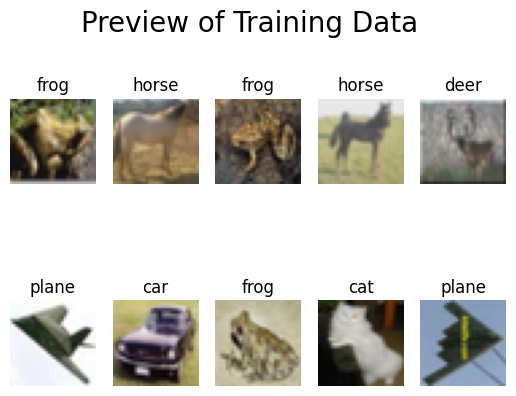
To make a good model, we need a great dataset. We’re using the CIFAR-10 dataset , which has 60,000 images, for our image classifier. Start by getting this dataset through torchvision and take a look at some of the images in it.
import torch
import torchvision
import torchvision.transforms as transforms
import matplotlib.pyplot as plt
import numpy as np

# Download the CIFAR-10 dataset to ./data
batch_size=10
transform = transforms.Compose([transforms.ToTensor(), transforms.Normalize((0.5, 0.5, 0.5), (0.5, 0.5, 0.5))])
print("Downloading training data...")
trainset = torchvision.datasets.CIFAR10(root='./data', train=True, download=True, transform=transform)
trainloader = torch.utils.data.DataLoader(trainset, batch_size=batch_size, shuffle=True, num_workers=2)
print("Downloading testing data...")
testset = torchvision.datasets.CIFAR10(root='./data', train=False, download=True, transform=transform)
testloader = torch.utils.data.DataLoader(testset, batch_size=batch_size, shuffle=False, num_workers=2)

# Model will recognize these kinds of objects
classes = ('plane', 'car', 'bird', 'cat', 'deer', 'dog', 'frog', 'horse', 'ship', 'truck')

# Grab images from our training data
dataiter = iter(trainloader)
images, labels = dataiter.next()

for i in range(batch_size):
    # Add new subplot
    plt.subplot(2, int(batch_size/2), i + 1)
    # Plot the image
    img = images[i]
    img = img / 2 + 0.5
    npimg = img.numpy()
    plt.imshow(np.transpose(npimg, (1, 2, 0)))
    plt.axis('off')
    # Add the image's label
    plt.title(classes[labels[i]])

plt.suptitle('Preview of Training Data', size=20)
plt.show()
Downloading training data...
Files already downloaded and verified
Downloading testing data...
Files already downloaded and verified
Step 2: Configure the neural network
Next, we’ll configure a neural network in PyTorch to turn images into descriptions using the dataset.
import torch.nn as nn
import torch.nn.functional as F
import torch.optim as optim

# Define a convolutional neural network
class Net(nn.Module):
    def __init__(self):
        super().__init__()
        self.conv1 = nn.Conv2d(3, 6, 5)
        self.pool = nn.MaxPool2d(2, 2)
        self.conv2 = nn.Conv2d(6, 16, 5)
        self.fc1 = nn.Linear(16 * 5 * 5, 120)
        self.fc2 = nn.Linear(120, 84)
        self.fc3 = nn.Linear(84, 10)
    def forward(self, x):
        x = self.pool(F.relu(self.conv1(x)))
        x = self.pool(F.relu(self.conv2(x)))
        x = torch.flatten(x, 1)
        x = F.relu(self.fc1(x))
        x = F.relu(self.fc2(x))
        x = self.fc3(x)
        return x
net = Net()

# Define a loss function and optimizer
criterion = nn.CrossEntropyLoss()
optimizer = optim.SGD(net.parameters(), lr=0.001, momentum=0.9)

print("Your network is ready for training!")
Your network is ready for training!
Understanding the Neural Network Architecture in PyTorch
The numbers in the PyTorch neural network layers are crucial for defining the architecture and determining the data flow through the network. Let’s break down each component:
Convolutional Layers (nn.Conv2d)
self.conv1 = nn.Conv2d(3, 6, 5): First convolutional layer. The numbers3,6, and5represent the number of input channels, the number of output channels, and the kernel size, respectively.3input channels suggest RGB input images. Outputs 6 feature maps with a 5x5 kernel.self.conv2 = nn.Conv2d(6, 16, 5): Second convolutional layer. Takes 6 output channels fromconv1and produces 16 output channels using a 5x5 kernel.
Pooling Layer (nn.MaxPool2d)
self.pool = nn.MaxPool2d(2, 2): Performs max pooling with a 2x2 window and a stride of 2, reducing the spatial dimensions of input feature maps by half.
Fully Connected Layers (nn.Linear)
self.fc1 = nn.Linear(16 * 5 * 5, 120): First fully connected layer.16 * 5 * 5calculates the number of input features.16is the number of output channels fromconv2, and5 * 5is the spatial dimension of each output channel. Outputs 120 features.self.fc2 = nn.Linear(120, 84): Second fully connected layer. Takes 120 features fromfc1and reduces them to 84 features.self.fc3 = nn.Linear(84, 10): Final fully connected layer. Takes 84 features and outputs 10 features, often corresponding to the number of classes in a classification task.
Important Note
The relationship between the layers is crucial. The output dimensions of one layer must match the input dimensions of the next. This is especially important for the first fully connected layer (fc1), where the input features must be correctly calculated based on the output shape of the preceding convolutional and pooling layers.
The formula for calculating the output size of each convolution or pooling operation is generally (W - F + 2P) / S + 1, where:
Wis the input size.Fis the filter size.Pis the padding.Sis the stride.
However, specifics like input image size and padding, essential for accurately calculating the dimensions, are not provided in the example.
Step 3: Train the network and save model
PyTorch improves network by tweaking its settings and testing how well it works with our labeled dataset.
from tqdm import tqdm

EPOCHS = 2
print("Training...")
for epoch in range(EPOCHS):
    running_loss = 0.0
    for i, data in enumerate(tqdm(trainloader, desc=f"Epoch {epoch + 1} of {EPOCHS}", leave=True, ncols=80)):
        inputs, labels = data

        optimizer.zero_grad()
        outputs = net(inputs)
        loss = criterion(outputs, labels)
        loss.backward()
        optimizer.step()

# Save our trained model
PATH = './cifar_net.pth'
torch.save(net.state_dict(), PATH)
Training...


Epoch 1 of 2: 100%|████████████████████████| 5000/5000 [00:20<00:00, 241.32it/s]
Epoch 2 of 2: 100%|████████████████████████| 5000/5000 [00:20<00:00, 239.70it/s]
Step 4: Test the trained model
# Pick random photos from training set
if dataiter == None:
dataiter = iter(testloader)
images, labels = dataiter.next()
# Load our model
net = Net()
net.load_state_dict(torch.load(PATH))
# Analyze images
outputs = net(images)
_, predicted = torch.max(outputs, 1)
# Show results
for i in range(batch_size):
# Add new subplot
plt.subplot(2, int(batch_size/2), i + 1)
# Plot the image
img = images[i]
img = img / 2 + 0.5
npimg = img.numpy()
plt.imshow(np.transpose(npimg, (1, 2, 0)))
plt.axis('off')
# Add the image's label
color = "green"
label = classes[predicted[i]]
if classes[labels[i]] != classes[predicted[i]]:
color = "red"
label = "(" + label + ")"
plt.title(label, color=color)
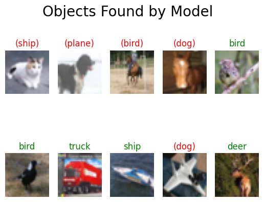
plt.suptitle('Objects Found by Model', size=20)
plt.show()
Step 5: Evaluate model accuracy
Finally, we’ll assess how well our model performs overall.
# Measure accuracy for each class
correct_pred = {classname: 0 for classname in classes}
total_pred = {classname: 0 for classname in classes}
with torch.no_grad():
    for data in testloader:
        images, labels = data
        outputs = net(images)
        _, predictions = torch.max(outputs, 1)
        # collect the correct predictions for each class
        for label, prediction in zip(labels, predictions):
            if label == prediction:
                correct_pred[classes[label]] += 1
            total_pred[classes[label]] += 1

# Print accuracy statistics
for classname, correct_count in correct_pred.items():
    accuracy = 100 * float(correct_count) / total_pred[classname]
    print(f'Accuracy for class: {classname:5s} is {accuracy:.1f} %')
Accuracy for class: plane is 55.8 %
Accuracy for class: car   is 56.2 %
Accuracy for class: bird  is 40.3 %
Accuracy for class: cat   is 25.0 %
Accuracy for class: deer  is 46.4 %
Accuracy for class: dog   is 40.8 %
Accuracy for class: frog  is 57.3 %
Accuracy for class: horse is 62.8 %
Accuracy for class: ship  is 69.7 %
Accuracy for class: truck is 61.6 %